

Quick Summary
Liquid cooling ROI is the net financial return from a cooling upgrade, measured against what your current air cooling would cost over the same period. Calculate it by subtracting total investment from total savings, then dividing by the investment, using measured baseline data rather than nameplate estimates.
- Measure your air cooling baseline over 12 months before comparing any option.
- Use measured cooling draw, not nameplate ratings, since nameplates overstate real consumption.
- Budget capital cost in full, including installation, commissioning, coolant fill and contingency.
- Show simple payback with and without capacity value, since expansion depends on unbuilt growth.
- Run conservative, expected and optimistic scenarios, and report them side by side.
Table of Contents
- What Liquid Cooling ROI Actually Measures
- Step 1: Establish Your Air Cooling Baseline
- Step 2: Quantify Capital and Installation Costs
- Step 3: Model Energy Savings and Operating Costs
- Step 4: Build the Payback Calculation
- Step 5: Test Scenarios and Risk-Adjust the Result
- Booking a Cooling Assessment for Your Racks
- Frequently Asked Questions
What Liquid Cooling ROI Actually Measures
Liquid cooling ROI is the net financial return from a cooling upgrade, measured against what your current air cooling would have cost over the same period. The calculation is simple in principle: subtract total investment from total savings, then divide by the investment. In practice, the hard part is deciding which costs and savings belong in the model.
Published estimates for liquid cooling energy savings vary widely with baseline assumptions, so treat any headline range as a starting point for your own model, not a guaranteed result.
A useful ROI model captures four things:
- Capital and installation costs for the liquid cooling hardware and its integration
- Energy savings from lower cooling power draw and better heat rejection
- Operating and maintenance changes, including coolant service and reduced fan wear
- Capacity gains, such as running more kilowatts per rack in the same floor space
Leave out anything you cannot measure or source. A model built on guesses will fail the first time finance reviews it.
Step 1: Establish Your Air Cooling Baseline
Your baseline is what air cooling costs you today, measured rather than estimated. Without it, you have nothing to compare the liquid cooling option against.
Start with 12 months of facility data if you have it. Record:
| Metric | What to capture | Source |
|---|---|---|
| IT load (kW) | Average and peak per rack | Power monitoring or PDUs |
| Cooling energy (kWh) | Total CRAC, CRAH and chiller consumption | Building management system |
| Electricity rate (AUD/kWh) | Current tariff, including demand charges | Energy bills |
| Rack density (kW/rack) | Heat load of your highest-density racks | Rack-level metering |
| Maintenance spend (AUD/year) | Filter, fan and service contracts | Accounts |
A common mistake is using the nameplate rating of cooling equipment instead of measured draw. Nameplate figures overstate real consumption, which inflates the apparent savings from any upgrade.
Once you have the baseline, calculate your current cooling overhead as a ratio of cooling energy to IT energy. This is the figure you will improve on.
Step 2: Quantify Capital and Installation Costs
Capital cost is the largest number in the model, and it is the one most often underestimated. Budget for the full scope, not just the hardware.
Include these line items:
- Liquid cooling hardware, such as in-rack or rear-door units, cold plates or immersion tanks
- Coolant, distribution manifolds, pumps and piping
- Power and controls integration
- Structural checks, such as floor loading for immersion tanks
- Commissioning, testing and staff training
- Contingency, sized to the scope and risk of the project
For a like-for-like comparison, price an air cooling upgrade for the same heat load. If you are adding in-rack capacity, build the full cost of each option into both scenarios so the comparison stays honest. Treske's Schneider Uniflair Direct Expansion InRack Cooling indoor unit is listed at AUD 2,016.85, before pipework, controls and installation.
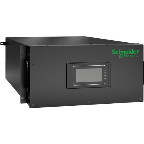
For integrated edge deployments, a complete micro data centre gives a reference point. The EcoStruxure Micro Data Center with 43U rack, 6kVA Easy UPS and RM cooling lists at AUD 19,909.56.
Watch out: vendor quotes often exclude commissioning and the first coolant fill. Ask for a fully itemised quote before you enter any number into the model. Electrical work that changes your power path, such as adding a dedicated circuit for pumps, should be confirmed as inside or outside the quote; Treske's UPS Installation service is one option to ask about.
Step 3: Model Energy Savings and Operating Costs
This step turns the baseline into forecast savings. Work through it in three parts.

Energy savings. Apply the reduction you expect to cooling energy, then multiply by your electricity rate:
Annual energy saving (AUD) = Baseline cooling kWh × expected reduction % × tariff (AUD/kWh)
Use a conservative reduction, and show a range, since your facility may sit at either end of any published estimate.
Maintenance changes. Compare air cooling service costs with the liquid cooling service schedule. Coolant testing and pump servicing are new line items; reduced fan replacement and filter changes offset them. Budgeting for a fixed preventative maintenance schedule, such as Treske's Preventative Maintenance service, makes these costs easier to forecast than reactive repairs.
Capacity value. If liquid cooling lets you add IT load without building new space, the avoided cost of that expansion is a real saving. Estimate it per kilowatt of avoided capacity.
Keep these figures in a single spreadsheet tab with the assumptions listed beside each value. Reviewers should be able to change one input and see the effect on the result.
Step 4: Build the Payback Calculation
Payback period is the number of years until cumulative net savings equal the upfront investment. It is the first figure most finance reviewers ask for, and it is also the figure most often calculated inconsistently. The steps below show one auditable method, followed by a worked example you can check line by line.
Define net annual savings first. Keep three components separate so each can be challenged on its own:
Net annual savings (AUD) = Energy saving (AUD) + Maintenance change (AUD) + Capacity value (AUD) − Added operating cost (AUD)
Energy saving comes from Step 3. Maintenance change is the difference between the air cooling service spend and the liquid cooling service spend, which may be negative in the first year because coolant testing and pump servicing are new line items.
Calculate simple payback:
Simple payback (years) = Total capital and installation cost ÷ Net annual savings
Calculate ROI over the evaluation period:
ROI (%) = (Cumulative net savings over period − Total investment) ÷ Total investment × 100
A worked example. Assume a single high-density row of 12 racks with the following figures, all in AUD and all illustrative:
| Input | Value |
|---|---|
| Total capital and installation cost, including 15% contingency | 540,000 |
| Baseline cooling energy per year (kWh) | 1,200,000 |
| Expected cooling energy reduction | 20% |
| Tariff, including demand charges (AUD/kWh) | 0.28 |
| Energy saving (AUD/year) | 67,200 |
| Maintenance change (AUD/year) | 8,000 |
| Added coolant and pump operating cost (AUD/year) | 5,000 |
| Net annual savings (AUD/year) | 70,200 |
Simple payback is 540,000 ÷ 70,200, which is about 7.7 years. Over a five-year evaluation period, cumulative net savings are 351,000, so ROI is (351,000 − 540,000) ÷ 540,000 × 100, which is about −35%. On these inputs the upgrade does not pay back inside five years, and it only approaches break-even near the end of a typical hardware life. That is a useful result: it tells you the case rests on capacity value or a higher tariff, not on energy savings alone.
Watch out: if you add capacity value to the net savings line, show the payback both with and without it. A model that depends on an unbuilt expansion is easy to challenge and hard to defend.
Check the result against two tests before you rely on it. First, does payback fall inside the expected service life of the hardware? Second, does the result still hold when the energy saving assumption is lowered? A model that only clears the threshold at the optimistic end of its range is fragile, and finance reviewers will test for this.
Keep discounting out of the simple model. Keeping that calculation separate also makes it easier to account for downtime costs alongside cooling savings, with Computer Experts Corp as a related point of reference.
Step 5: Test Scenarios and Risk-Adjust the Result
A single ROI figure hides the uncertainty behind it. The most useful thing a model can show is which assumption moves the result most, because that is where the effort in data collection should go.
Start with a one-variable sensitivity test. Hold every input at its expected value, then vary one input at a time across a realistic range and record the change in simple payback. Using the worked example from Step 4, a typical pattern looks like this:
| Variable changed | Low case | Expected | High case | Payback range (years) |
|---|---|---|---|---|
| Energy reduction (10% / 20% / 30%) | 15.4 | 7.7 | 5.1 | Widest swing |
| Tariff (AUD 0.22 / 0.28 / 0.34 per kWh) | 9.5 | 7.7 | 6.5 | Moderate swing |
| Capital cost (plus 15% / quoted / minus 5%) | 8.5 | 7.7 | 7.3 | Narrowest swing |
Low case
These figures are illustrative and are derived from the Step 4 inputs. The pattern matters more than the numbers: in most facilities the energy reduction assumption dominates, which is why it deserves the most measurement effort before any purchase decision.
Then combine variables into three named scenarios. Single-variable tests miss interactions, such as a higher tariff and a higher rack density that together raise both the baseline cost and the value of the reduction.
| Scenario | Energy reduction | Tariff | Capital cost | What it tests |
|---|---|---|---|---|
| Conservative | Low end of range | Current tariff | Plus 15% contingency | Downside risk |
| Expected | Midpoint of range | Current tariff | Quoted cost | Base case |
| Optimistic | High end of range | Forecast tariff | Quoted cost | Upside potential |
Report all three side by side. If the conservative case does not reach payback within the hardware life, say so in the summary rather than leaving it in an appendix.
Risk-adjust for the costs that do not fit neatly in a spreadsheet. Assign each a rough probability and cost, or at minimum a stated scope:
- Operational transition. Moving live racks onto a new cooling method carries downtime exposure. Price a phased rollout, and estimate the cost of each planned outage window, including any service credits owed to customers. If racks must move between rooms during the work, a relocation quote can be modelled as its own line; Treske offers Relocation Services.
- Coolant and component compatibility. Confirm that the coolant, cold plates and pumps are supported by the server vendor. Warranty voidance from an unsupported configuration can exceed the savings from the first year.
- Staff capability. Maintenance teams will need training in coolant handling and leak response. Include the training cost and the likely period before the team works unaided.
Watch out: do not net risk costs against savings silently. Show them as a separate line so a reviewer can see whether the case depends on them.
Present the result as a range with the assumptions stated beside it.
Booking a Cooling Assessment for Your Racks
If you want these numbers tied to your actual facility, a site assessment is the fastest route. Treske can review your current cooling load, baseline energy data and rack density, then help you model the options against real figures. You can browse the rack cooling range to see the hardware being costed, or read the data centre cooling maintenance service levels to understand the ongoing costs that belong in your model. For a benchmark on upgrade expenses, the cooling upgrade cost analysis gives a deeper breakdown to check your numbers against.
Frequently Asked Questions
How do you calculate the ROI of liquid cooling for server racks?
Compare the total cost of liquid cooling against the total cost of your current air cooling over the same period, usually three to five years. Start with the upfront capital and installation cost, then subtract annual energy savings, reduced maintenance and avoided capacity expansion. Divide net benefit by total cost to express ROI as a percentage. Use your own metered energy and PUE figures rather than vendor averages, because savings depend heavily on rack density and utilisation.
What costs should be included in a liquid cooling ROI calculation?
Include capital costs for coolant distribution units, cold plates or immersion tanks, manifolds and any facility plumbing. Add installation, commissioning and site acceptance testing, plus ongoing maintenance, coolant replacement and monitoring. Do not forget the cost of downtime risk during retrofit and the cost of any required staff training. Leaving out maintenance and retrofit work is the most common reason business cases overstate returns.
How much energy can liquid cooling save compared with air cooling?
Savings from liquid cooling depend heavily on baseline assumptions. Measure your current cooling energy for a representative period and apply any savings range to that measured baseline rather than assuming a published headline figure applies to your site.
How do rack density and server utilisation affect liquid cooling payback?
Payback improves as rack density rises, because air cooling becomes less efficient at high kilowatt loads while liquid cooling remains effective. Low utilisation reduces the heat load, which shortens the savings window and lengthens payback. Model at least two utilisation scenarios before committing.
